

Second Order Probabilities
Creation of a high-fidelity, analytical resilience metric suffers the non-idealities inherent in most engineering activities. Engineers consistently bump up against the unknowable when constructing models and building and measuring hardware and its performance. Many of these error contributors are referred to as “second-order” or “third-order” effects because their impact on the final result is much less than the “first-order effects.”. Noise and interference, atmospheric effects on communications signals, and small parasitic capacitances and inductances are examples of this. Likewise, the reliability of functional blocks in a system represent another form of uncertainty. Often this is not due to the system design but rather an inhospitable and random operational environment. An effect which may have significant impact or consequence, but much lower probability of occurrence could also be considered a “second-order effect,” or a “second-order probability.” It may not be credible in some instances, but the designer may need or want to consider them in others, particularly if margin is at a premium.
The fundamental resilience equation in my book relies on four parameters based upon four resilience attributes. Only one of those, avoidance, is expressed as a probability. This is because of the uncertainty associated with both the threat effectiveness and the mitigation effectiveness. Strictly speaking these parameters are not reliability values as they are not driven by component or system failures, but rather the fact that the techniques have some probability of not being successful. When combined the two can be represented as a probability of avoidance.
The other three parrameters in the equation, robustness, recovery, and reconstitution, are presented in the book as deterministic values. This was intentional partly because in most cases this will be true, and partly to simplify the examples in an introductory text. However, this need not be the case, and there are simple analytical methods to accommodate these cases. Of course, this assumes that a credible probability can be assigned to these parameters, based upon measurement or some other analytical forecasting method, including statistical means.
An example is a system element that features an autonomous recovery mechanism to recover lost capability after a threat has caused a loss. In the simplest case the recovery metric is a fixed value based upon the recovery level and recovery time and assumes that the recovery will execute when activated. If there is some quantifiable, non-zero probability that the recovery feature will not function when activated then there are two outcomes possible: the recovery activates and the expected recovery function is successful, or the recovery does not occur and the metric is zero.
To incorporate this into the resilience metric requires simply another expected value calculation based upon the two outcomes. This is identical to the calculation used to incorporate the probability of avoidance into a capability response using the expected value and the probability of avoidance. Here a new variable is introduced, the probability of recovery. The new, probability-adjusted recovery metric RAV’ can be found by:
RAV’ = [PAV][RAV] + [1-PAV][0] = [PAV][RAV]
Thus the probability of recovery scales the ideal / nominal recovery metric, with PAV constrained to values of 0 and 1 inclusive. In the same way that the probability of avoidance can be used to scale the non-avoided capability response profile, so can a probability of recovery be used to further scale the recovery portion of the same response. A probability of robustness and a probability of reconstitution could also be created and applied to both the capstone equation variables as well as scaling of the applicable portions of a capability response.
An example is shown in the figure below. A probability of recovery value of 0.75 adjusts the nominal value of RAV = 0.3. The adjusted value of the recovery metric is 0.225 due to a 25% reduction in the final recovery level value. The accompanying capability response shows how the probability of recovery is used to scale the recovery level from 0.8 (the case in which recovery occurs) to 0.65 when considering a 25% chance that recovery fails. The associated resilience values for both cases, unadjusted and adjusted, are also provided. Note that this adjustment is independent of the probability of avoidance, both can be applied to the same capability response. Note that the recovery time does not change, as it is not dependent in any way upon the probability of recovery. If recovery occurs, it occurs at t = 0.6.
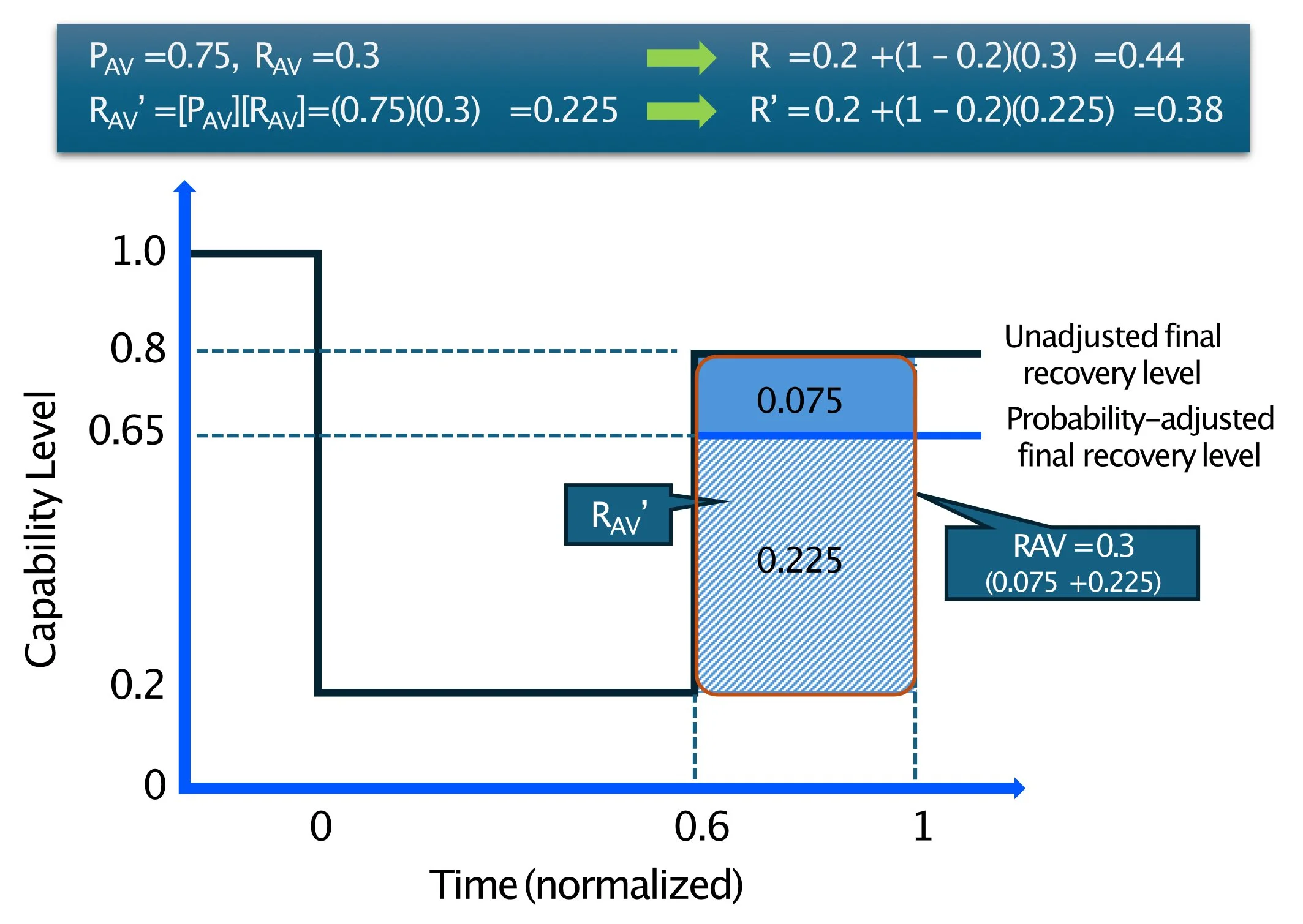
Example of the use of a probability of recovery to adjust the nominal recovery metric, including adjustment to capability response values